The Mosaic Image

The IMA2 level produces JEM-X mosaic images by combining all the individual j_ima_iros images from the different science windows gathered in the observation group. The combined images have longer exposure time. As a consequence, weaker sources which are not visible in single ScW may appear in the mosaic images.

In what follows we consider an example of a JEM-X mosaic of the Galactic Center region for the revolution 0053 in March 2003. You can browse through the INTEGRAL data archive and check that within this revolution the pointings which have the Galactic Center within the JEM-X2 FOV are

005300410010.001
005300420010.001
005300490010.001
005300510010.001
005300580010.001
005300590010.001
005300650010.001
005300660010.001
005300670010.001
005300680010.001
005300740010.001
005300750010.001
005300760010.001
005300820010.001

Save the above list to the file mos.lst. To produce the mosaic image of these pointings you have first to create the corresponding observation group mos using the og_create tool, as has been explained above, and run the jemx_science_analysis up to the IMA level.

cd $REP_BASE_PROD
og_create idxSwg=mos.lst ogid=mos baseDir="./" instrument=JMX2
cd obs/mos
jemx_science_analysis startLevel="COR" \
   endLevel="IMA" nChanBins=-1 jemxNum=2

Next, to produce the mosaic from the intensity images for each energy band as obtained at the IMA level, you have to run the jemx_science_analysis script at IMA2 level only:

jemx_science_analysis startLevel="IMA2" endLevel="IMA2" jemxNum=2

Again, do not forget to specify which of the JEM-X instruments you are interested in (jemxNum=2 in our case). By default, ``intensity'' (RECONSTRUCTED), ``variance'', ``significance'' and ``exposure'' mosaic images will be produced.

The same result can be obtained calling jemx_science_analysis only once, from startLevel="COR" to endLevel="IMA2", eventually skipping the intermediate levels with the command skipLevels="LCR, SPE, BIN_S, BIN_T".

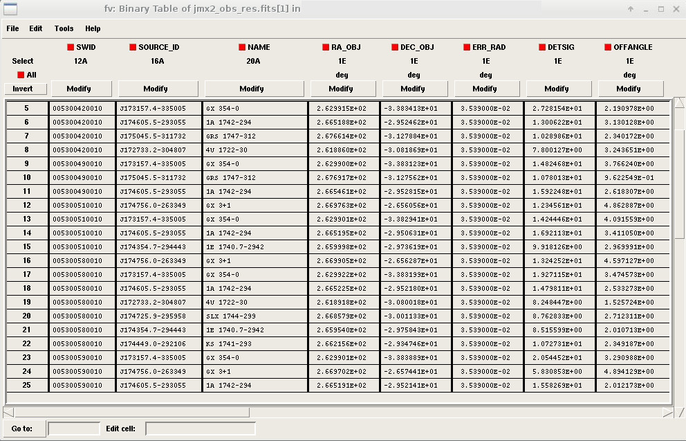
Apart from the mosaic images, the output of the IMA2 level contains a collection of the results from the individual science windows. The file jmx2_obs_res.fits lists all sources found in individual science windows with the respective fluxes and significances. A part of its content is shown as an example in Fig. .

Figure: Part of the content of jmx2_obs_res.fits file.

With the help of cat2ds9 command you can produce a region file found.reg to locate these sources at the mosaic image:

cat2ds9 jmx2_obs_res.fits\[1] found.reg symbol=circle color=white

Note that since the same sources can be found in many ScWs you can have one and the same source repeated several times in the resulting region file.

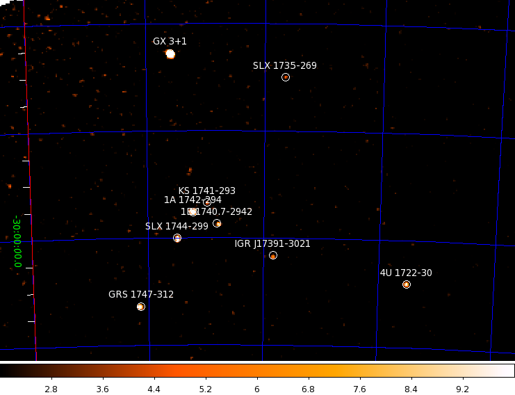
You can look at the content of the resulting mosaic images contained in the file jmx2_mosa_ima.fits with fv and display them with ds9 exactly as you did with the images from individual ScWs. With the command

ds9 jmx2_mosa_ima.fits\[4] -region found.reg

and some additional aesthetic adjustments you can obtain an image as the one in Fig. , which displays the significance map in the 3-10 keV energy band. The sources found in single ScW analysis are shown with white circles.

Figure: The mosaic image of the Galactic Center region for revolution 0053 in the 3-10 keV energy band (significance map).

If you are interested only in a particular region of the mosaic you can ``zoom'' on a given position in the sky running jemx_science_analysis with additional parameters IMA2_RAcenter, IMA2_DECcenter and IMA2_diameter which will specify the position of the center and the diameter (in degrees) of the resulting mosaic image. To do so, first move the existing images:

mv jmx2_mosa_ima.fits jmx2_mosa_ima_original.fits
mv jmx2_obs_res.fits jmx2_obs_res_original.fits

Remember that the images have to be also removed from the observation group. This can be done by the following command:

dal_clean og_jmx2.fits+1

Now re-run the analysis script:

jemx_science_analysis startLevel="IMA2" endLevel="IMA2" jemxNum=2 \
   IMA2_diameter=5.0 IMA2_RAcenter=266.4 IMA2_DECcenter=-29.0

(we have chosen to center the image on the Galactic Center position here).

If you want to produce a mosaic image only for a specific energy band you can pass the minimal and maximal energies of the selected energy band to the jemx_science_analysis through the parameters IMA2_eminSelect and IMA2_emaxSelect. Note that the energies have to be the same as defined previously in chanLow and chanHigh.

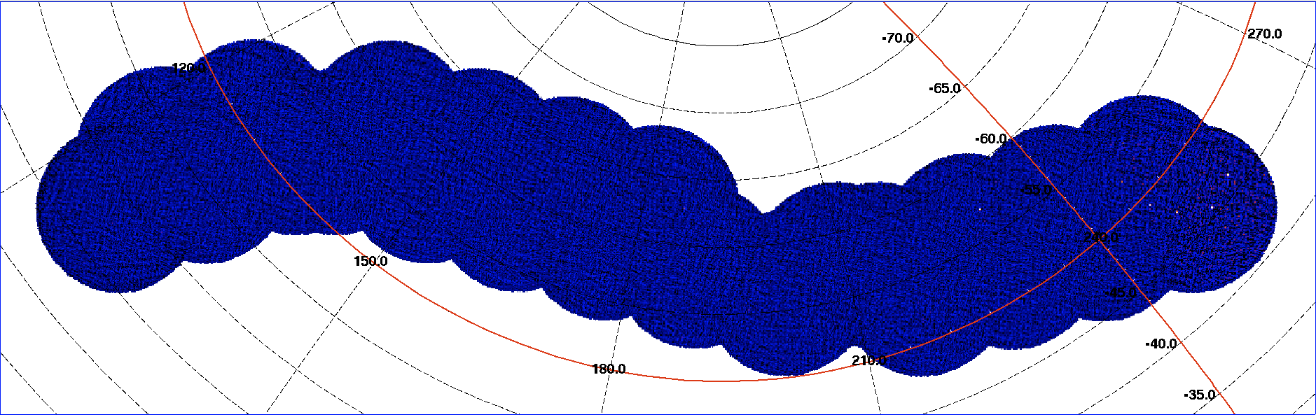
To get the largest possible output mosaic in equatorial coordinates the parameters "radiusSelect" and "diameter" must both be set to -1. A better way, available with OSA v.10.0, is to use the Aitoff-Hammer projection (in galactic coordinates) by setting the option AITproj. The latter enables the mosaicking of large parts of the sky, such as for the Galactic Plane Scans, without distortion of the map (an example is in Fig. ). This new feature can be activated setting the parameter IMA2_AITproj="yes". The command should be therefore as follows:

jemx_science_analysis startLevel="IMA2" endLevel="IMA2" jemxNum=2 IMA2_AITproj="yes"

The resulting AIToff mosaics are expected to be mapped in the Galactic plane, and are therefore oriented in galactic, rather than equatorial, coordinates. To produce a mosaic over the whole sky you will need to decrease the resolution of the image by increasing the pixel size (cdelt) at least to 0.075 degree. The computation in AIToff-Hammer projection can take approximately 10% more CPU-time; and the resulting file can have a rather large dimension (for example 1G). In this case a simple solution can be to compress the file (e.g. with gzip) and to work directly with the compressed file (ds9 as well as other HEASOFT tools are able to work directly with the compressed file).

Figure: The mosaic image of the Galactic Plane Scan observation of revolution 399 in the 3-10 keV energy band, obtained in AIToff-Hammer projection.