Results from the Image Step

After jemx_science_analysis finishes its operation, the results are stored separately for each ScW of the observation group. They are located in the subdirectories named scw/RRRRPPPPSSSF.001/ (where RRRRPPPPSSSF is the number of the ScW).

Go to one of these directories and have a look at the files

cd scw/010200210010.001/
ls

This is the output from all the processing steps done by the script.

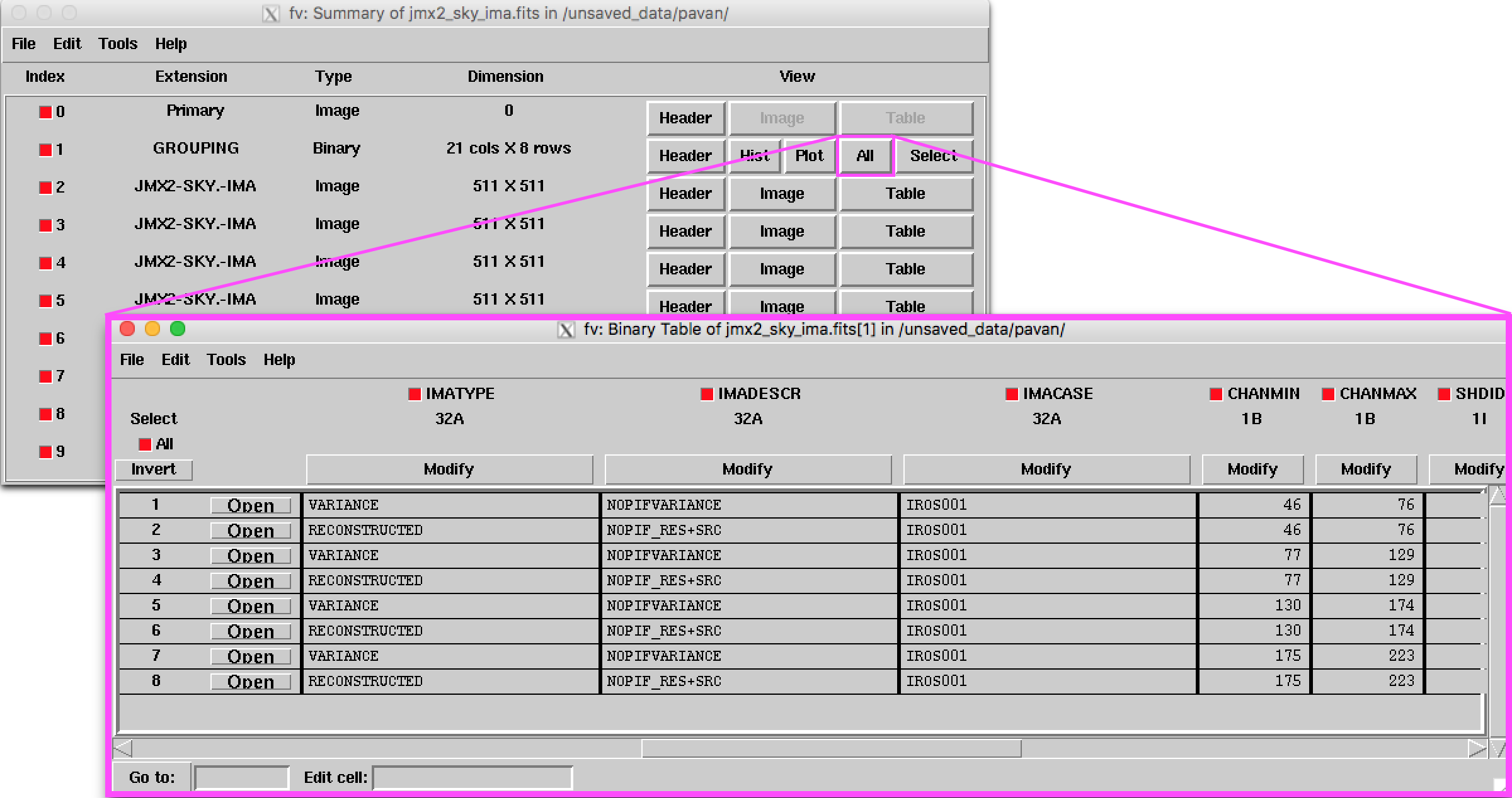
The output image is jmx2_sky_ima.fits. You can check it using e.g. fv:

fv jmx2_sky_ima.fits

You will find that this file contains 9 extensions: the index of all images, 4 cleaned sky images (RECONSTRUCTED type), and 4 variance maps, one for each of the 4 selected energy bands (see Fig. ).

Figure: The content of jmx2_sky_ima.fits file.

In the file jmx2_srcl_res.fits you find a list of all found sources, the energy bands, and the derived flux values. The detection significance is the maximum one between the energy bands. The E_MIN, E_MAX, FLUX, FLUX_ERR arrays contain the energy bands of your choice plus the three standard ones used internally by the software. They can be visualized using fv and clicking on "modify" under the column name and then "expand" on the scroll-down menu. and in the file jmx2_srcl_cat.fits the list of the sources in the input catalog. You can see that most of the catalog sources were not found, as they are too weak. When you run the lightcurve and spectra extraction steps the results would be produced for all sources listed in jmx2_srcl_res.fits.

WARNING: Since OSA v.10.0 images are produced with counts per cm . Since OSA v.10.1 source spectra and lightcurves show (again) countrates per unit of detector area (100 cm ), in agreements with OGIP standards requirements. To extract the correct source fluxes you must use OSA version 10.1 or later with the latest available IC files.

There is a nice way to locate the found sources as well as the catalog sources on the sky image. To do it use the utility cat2ds9:

cat2ds9 jmx2_srcl_res.fits\[1] found.reg symbol=box color=red
cat2ds9 jmx2_srcl_cat.fits\[1] cat.reg symbol=circle color=white

(to find out more about this program type cat2ds9 -h in the command line). With the help of the above two commands the two files found.reg and cat.reg are created. They contain the lists of all the found sources and all the catalog sources, respectively.

With the help of the ds9 viewer you can display the sky images in any of the available energy bands. For example, to look at the 5-10 keV reconstructed image which (if you used the option IMA_userImagesOut=yes) is contained in the 5th extension of the jmx2_sky_ima.fits file you can type

ds9 jmx2_sky_ima.fits\[5] -region cat.reg jmx2_sky_ima.fits\[5] -region found.reg

This command loads the region files cat.reg and found.reg created with cat2ds9. This can be done also using the ``Region'' menu of ds9.

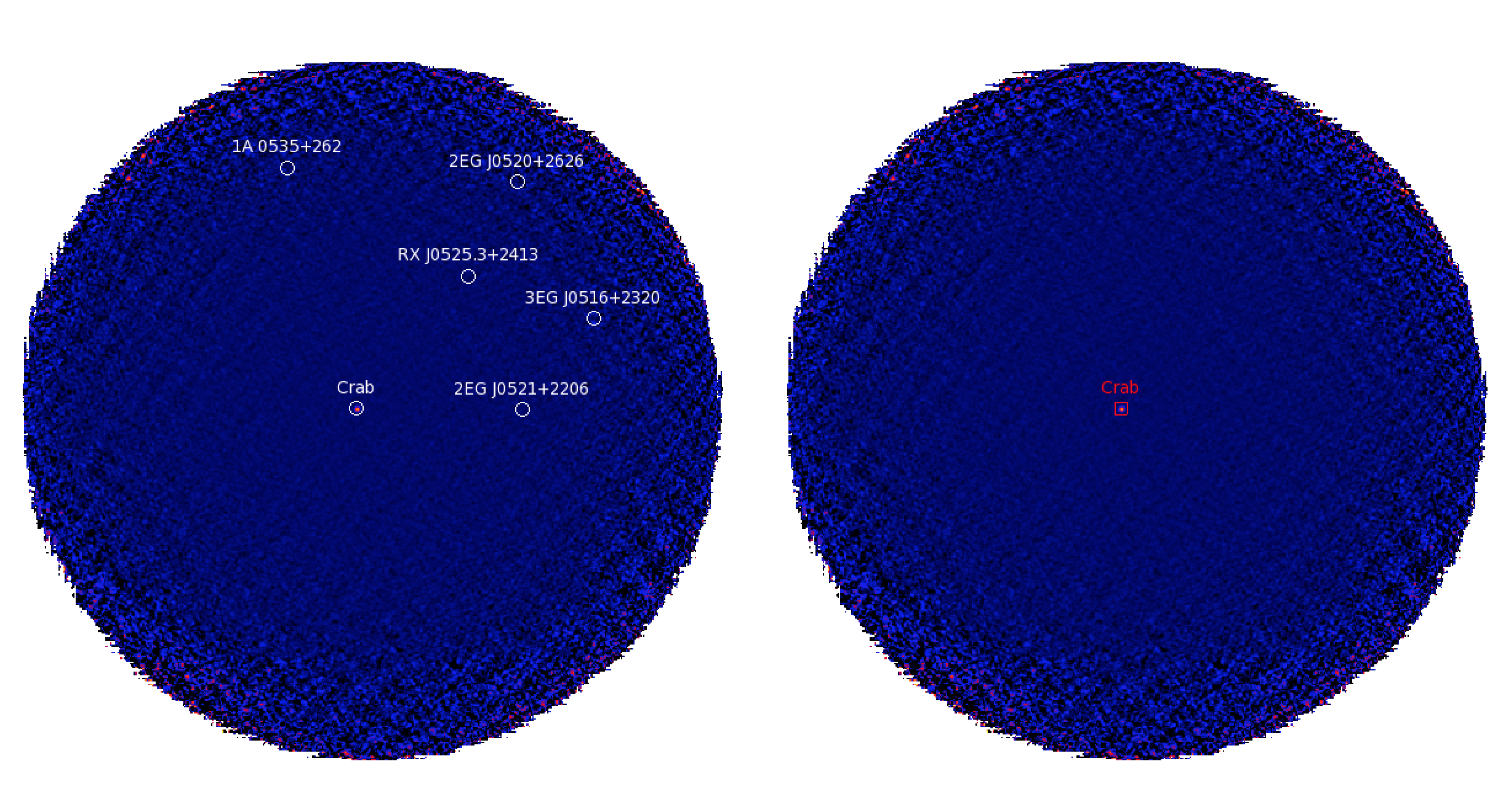
In Fig. , the left panel shows the Crab region in the second energy band (5-10 keV) with the catalog sources, and the right one - the same region with the found sources (Science Window 010200210010).

Figure: The image of Crab region. Catalog sources in the FOV are shown with white circles. The only found source (Crab) is shown with a red box.