Light-curves

Spiros can only produce light curves for sources provided through an input catalogue. The easiest starting point in this cook book is to copy the data set used for ``imaging with a catalogue'' for which we used a single energy bin from 20-40 keV. The commands below will save the results of spectral analysis and start again with the imaging data set (note that the below naming is somewhat arbitrary, working directly in a spi_timing directory could also be meaningful).

cd ..
mv spi_analysis spi_spectra
cp -r spi_imaging_with_catalogue spi_analysis
cd spi_analysis

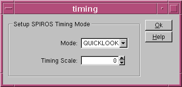
Launch ``spi_science_analysis'', check that an input catalogue is provided and un-select all tasks except spiros. Open the ``Spiros options'' GUI and set the spiros mode to TIMING. Click on the timing button to get the timing GUI.

Figure: spiros timing mode GUI

Set the mode to QUICKLOOK and the Timing Scale to 0. The Timing Scale is the time resolution of the resulting light curve in days. Setting it to 0 will give you one data point per science window (at the moment it is not possible to create light curves with a resolution smaller than one science window. ). Click ``Ok'' twice and then ``Run''.

Figure: Crab light-curve from the cookbook example

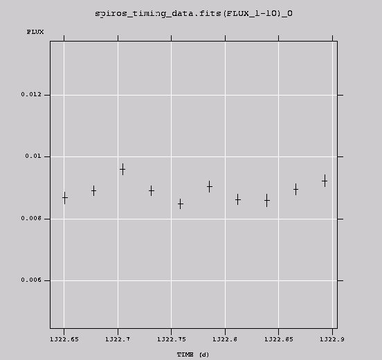
The resulting light-curve is written to spiros_timing_data.fits. This file contains one extension for each source plus the background (first data extension). This light-curve can be displayed with, e.g., ``fv'' to produce the output presented in Fig. .