Individual Science Windows Spectra

Let us first proceed with the spectral extraction using the source positions found at the IMA step. In our example only the Crab was found by the imaging analysis, so the spectral analysis will generate only the spectrum of the Crab if you run the script with default values (assuming you run j_rebin_rmf in your $REP_BASE_PROD directory).

We are now interested in extracting the spectra in a number of energy bands different from the ones used for the IMA step in the previous example. In this case we start a new analysis from COR level with the desired energy bands for spectral analysis.
If during your analysis the energy bins used to extract images and spectra are the same, you can continue the spectral analysis from the same og_group where you previously run the IMA step, by launching jemx_science_analysis with startLevel=''SPE'' and endLevel="SPE".

cd $REP_BASE_PROD
og_create idxSwg=jmx.lst ogid=crab_spec baseDir="./" instrument=JMX2
cd obs/crab_spec

jemx_science_analysis startLevel="COR" endLevel="SPE" \
   response="$REP_BASE_PROD/jmx2_rmf_mybins.fits" nChanBins=-4 \
   jemxNum=2

The results of the spectral analysis data are in the file

scw/RRRRPPPPSSSF.001/jmx2_srcl_spe.fits

Look on the result of the spectral analysis of the Science Window 010200210010

cd scw/010200210010.001/
fv jmx2_srcl_spe.fits

In this file, you find the spectra for all sources that were found at the IMA level.

Figure 19: Left panel: Crab spectrum in ScW 010200210010. Right panel: Combined Crab spectrum of ScW 010200210010 and ScW 010200220010.

The JEM-X systematics are of the order of a few percents, typically 3%. We add this explicitly to jmx2_srcl_spe.fits file with the command below:

fparkey 0.03 jmx2_srcl_spe.fits SYS_ERR add=yes

The obtained spectrum can be analysed e.g. within XSPEC program:

xspec
XSPEC>cpd /xw
XSPEC>data jmx2_srcl_spe.fits{1}
XSPEC>ign **-3.0 20.0-**
XSPEC>setplot energy
XSPEC>model po
XSPEC>fit
XSPEC>plot ldat del
XSPEC>quit

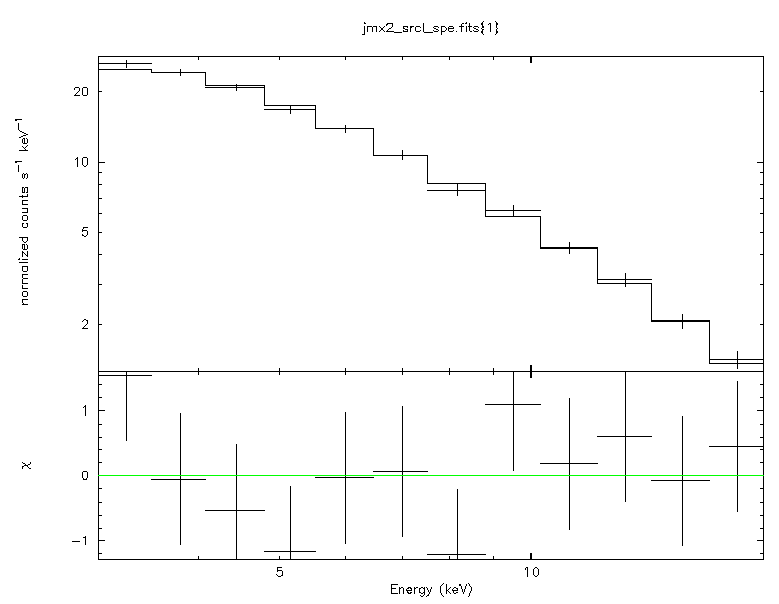
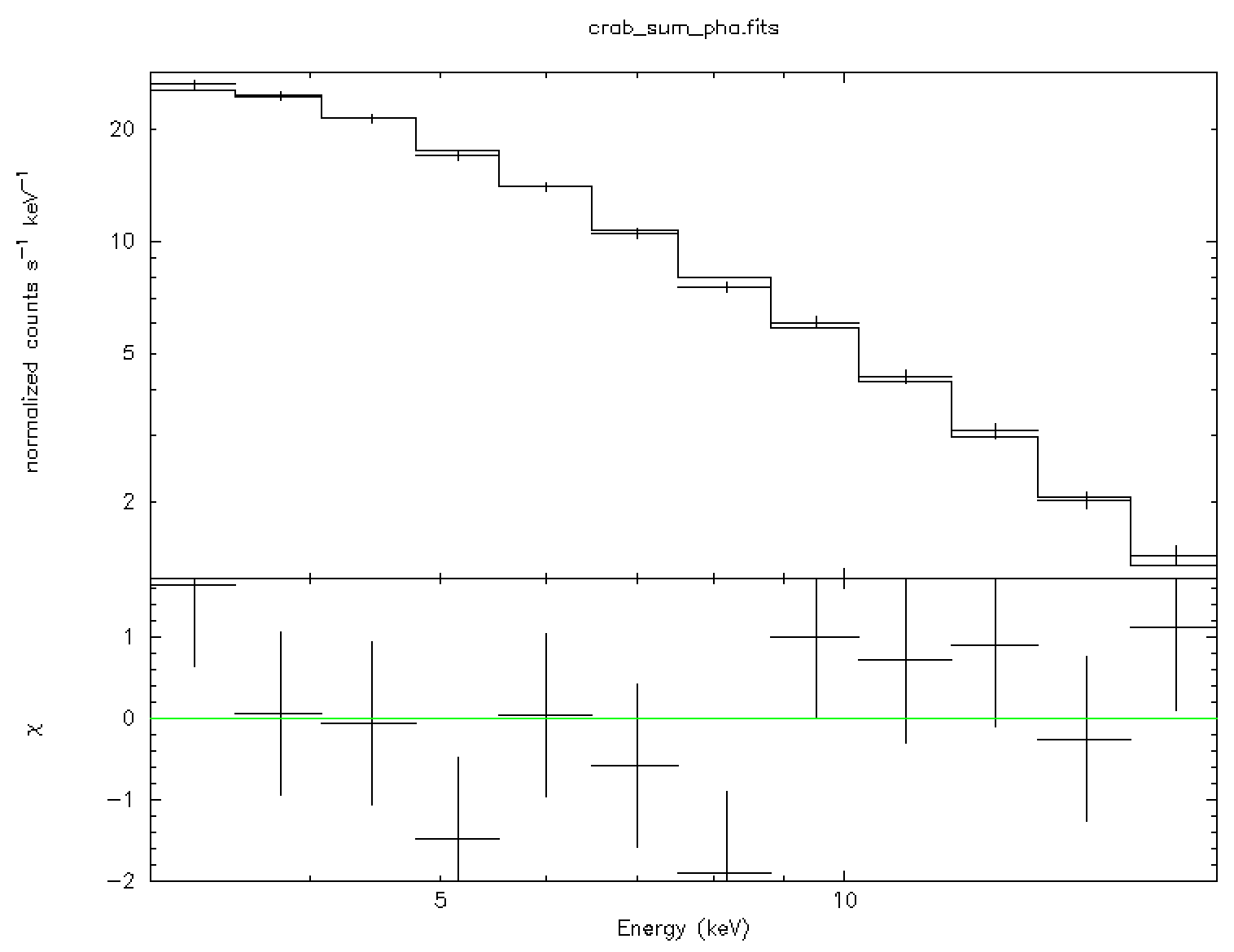
The above set of XSPEC commands reads the data file and fits the data with ``power-law'' model. The result is shown in the left panel of Fig. 19.

To understand the importance of the ``user catalog'', let us extract the Crab spectrum using the catalog position of the source, not the one found at the IMA level. To create the catalog for our source of interest, the Crab, one can just copy the corresponding line from the general reference catalog:

fcopy "${ISDC_REF_CAT}[NAME=='Crab']" user_cat.fits

In the new user_cat.fits file you have to change the FLAG column to 1; this is the last column of the file, not to be confused with the JEMX_FLAG for instance. In this case, jemx_science_analysis will directly copy the source position information to the jmx2_srcl_res.fits after IMA step (see Sections 6.8.6 and 10.6.1 for an explanation on the possible FLAG values).

Then, you have to re-run the analysis starting from the very beginning, but specifying that you want to use your own catalog for the spectral and lightcurve extraction. Create a new observation group crab_usrcat

cd $REP_BASE_PROD
og_create idxSwg=jmx.lst ogid=crab_usrcat baseDir="./" instrument=JMX2

copy the user catalog created as explained above into the observation group

cp user_cat.fits obs/crab_usrcat

and run the analysis up to the SPE level in this group:

cd obs/crab_usrcat
jemx_science_analysis startLevel="COR" \
   endLevel="SPE" jemxNum=2 CAT_I_usrCat="user_cat.fits" \
   nChanBins=-4 response="$REP_BASE_PROD/jmx2_rmf_mybins.fits"

The obtained spectra can be analysed with XSPEC as it was done above. Differences are generally marginal, but they might become more important for a weak source in a crowded region, where the fitted position might be significantly different from the real one.