It is convenient to look at the images with the help of the ds9 program. First create a region file from the catalog using the cat2ds9 program. In the example below we create the region file found.reg with all the sources found in the mosaic image, isgri_mosa_res.fits, for the first energy band (extension [2]), and a region file cat.reg with all sources that were in the input catalog isgri_catalog.fits.
cd $REP_BASE_PROD/obs/isgri_gc
cat2ds9 isgri_mosa_res.fits\[2] found.reg symbol=box color=green
cat2ds9 isgri_catalog.fits cat.reg symbol=box color=white
To see the resulting images:
ds9 $REP_BASE_PROD/obs/isgri_gc/isgri_mosa_ima.fits\[2] \
    -region $REP_BASE_PROD/obs/isgri_gc/cat.reg \
    -cmap b -scale sqrt -scale limits 0 60 -zoom 2 \
    $REP_BASE_PROD/obs/isgri_gc/isgri_mosa_ima.fits\[4] \
    -region $REP_BASE_PROD/obs/isgri_gc/found.reg \
    -cmap b -scale sqrt -scale limits 0 60
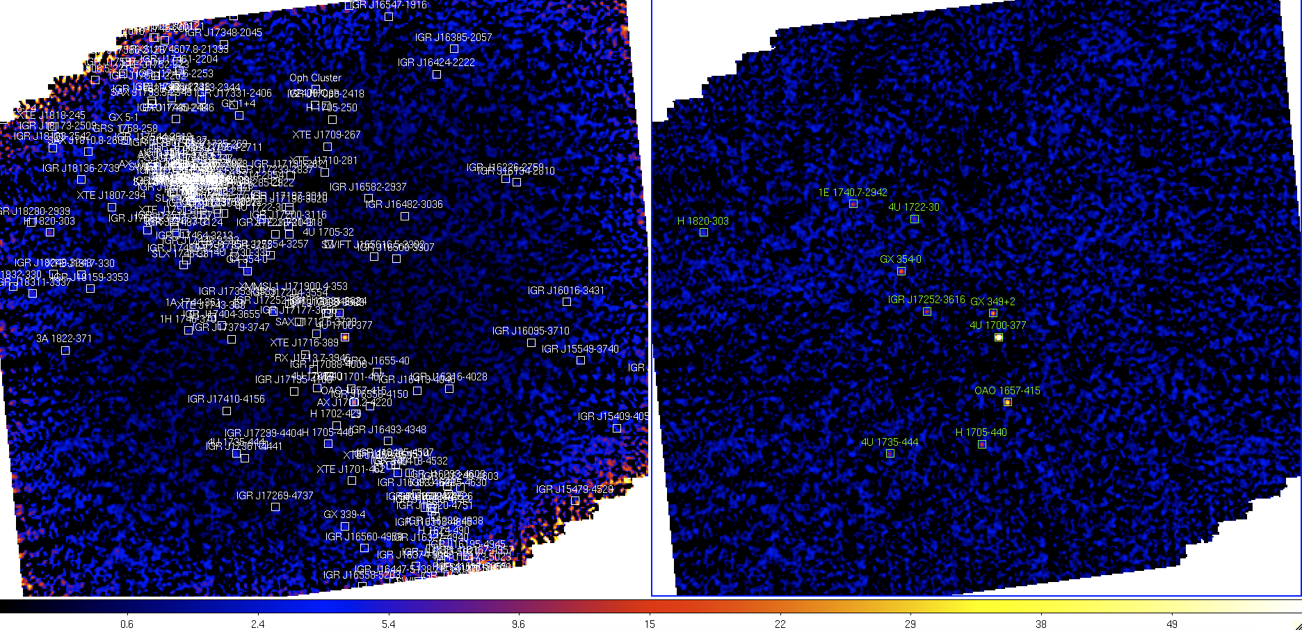
In Figure ![[*]](crossref.png) you see the INTENSITY
(left, $REP_BASE_PROD/obs/isgri_gc/isgri_mosa_ima.fits[2])
and the SIGNIFICANCE
(right, $REP_BASE_PROD/obs/isgri_gc/isgri_mosa_ima.fits[4])
mosaic images in the 20-40 keV energy range. In the left
image we have shown all catalog sources (white boxes), and in the
right one only the detected ones (green boxes).
The color scale at the bottom gives the significance values.
Although we used here a square-root scaling (sqrt) that enhances
the structure in the low-values (the background) we now have a very clean
mosaic image compared to images obtained with OSA versions prior to OSA 9.
The issue of spurious new sources detected by the software at the position
of the ``ghosts'' of true sources is therefore much reduced.
you see the INTENSITY
(left, $REP_BASE_PROD/obs/isgri_gc/isgri_mosa_ima.fits[2])
and the SIGNIFICANCE
(right, $REP_BASE_PROD/obs/isgri_gc/isgri_mosa_ima.fits[4])
mosaic images in the 20-40 keV energy range. In the left
image we have shown all catalog sources (white boxes), and in the
right one only the detected ones (green boxes).
The color scale at the bottom gives the significance values.
Although we used here a square-root scaling (sqrt) that enhances
the structure in the low-values (the background) we now have a very clean
mosaic image compared to images obtained with OSA versions prior to OSA 9.
The issue of spurious new sources detected by the software at the position
of the ``ghosts'' of true sources is therefore much reduced.
Indeed, in a coded mask instrument with a symmetric mask pattern as in the case of IBIS
a true point source will cause secondary
lobes, 8 main ``ghosts'' aligned with the detector edges, at a distance
that is a multiple of the mask basic pattern, 10.7 degrees in
IBIS/ISGRI case (cf. Figures and ).
The ``ghosts'' of sources detected in individual ScW images will be removed
from these images and will thus not affect the mosaic image.
However, if a source is too weak to be automatically detected in a single ScW,
its ghosts are not cleaned, they can appear in the mosaic image and even
be found by the software as new sources.
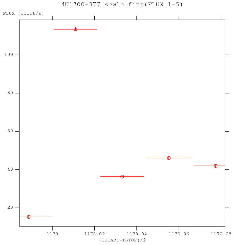
There is an easy way to collect from different ScWs all the
information related to a given source and energy band. In the example
below we create a file 4U1700-377_scwlc.fits with all the
information on 4U 1700-377 in 20-40 keV energy band. The structure
of this file is explained in Appendix , Table
.
src_collect group=og_ibis.fits+1 results=4U1700-377_scwlc.fits \
                  instName=ISGRI select="NAME == '4U 1700-377' && E_MIN==20"
In Figure the ScW-per-ScW lightcurve of 4U 1700-377 in the 20-40 keV band is shown. A ligthcurve with a finer time binning can be constructed at the LCR level (see Sect. ).
Note that the count rates are already corrected for instrumental effects such as the off-axis transparency of the mask supporting structure.