Gamma Ray Burst imaging

In the following cookbook section we explain how to derive images of short bursts, such as GRB, from SPI data. We assume that readers have some knowledge about SPI data analysis with the ISDC spi_science_analysis script. Please follow the above cookbook example if it is not the case.

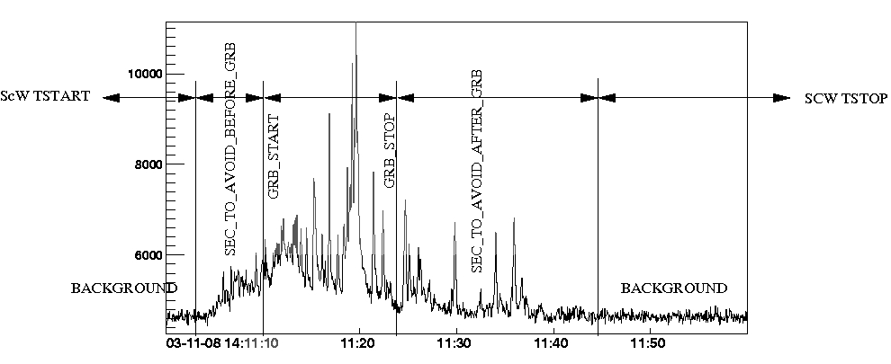
1. The first step is to record the start (grb_start) and stop (grb_stop) times of the period you want to use to derive the image, and possibly the time before (sec_to_avoid_before_grb) and after (sec_to_avoid_after_grb) the burst that should not be included in the period used to derive the background. Times can be in UTC or IJD. The best way to look at the timing is to display the burst light curve, for example using the SPI/ACS data. Of course, you can repeat the analysis in as many time bins as you wish, e.g., to derive a set of images and a SPI light-curve. Figure  provides an illustration of the required times on top of a real GRB light-curve.

   Figure: Illustration of the different GRB start/stop times

   

2. Set up your analysis environment as indicated in the "Setting up the analysis environment" section of the SPI data analysis cookbook.

3. Identify the pointing encompassing the burst, and use og_create to build an observation group (only analysis of a single pointing are possible in this frame), as shown in Fig. .

   Figure: Output of og_create on the terminal

   

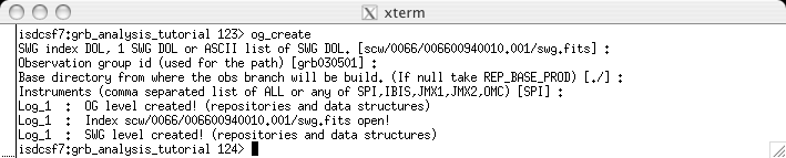
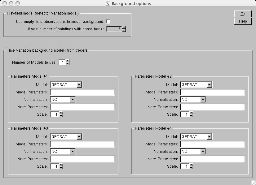
   This produces an observation group with a standard name "og_spi.fits" (located in ./obs/grb030501/ in our example).

4. Move to the observation group location (cd obs/grb030501 in our example).

5. The simplest to specify the parameters of your analysis is to use spi_science_analysis GUI:
   1. Run "spi_science_analysis" and specify parameters through the GUI, as displayed in Fig. .

      Figure: Main GUI window of the spi_science_analysis script

      

   2. Make sure that the ``catalogue extraction'' is un-selected, and that no ``spiros Input Catalogue'' is provided (in this imaging example we assume that the GRB position is unknown).

   3. Check the "List of detectors" (use 0-18 in most cases) and the ``Coordinate System'' in that window and click on "Energy_definition" to open the GUI window (see Fig. ).

      Figure: Energy boundaries (or ebounds) GUI

      

   4. Select your energy bins (in principle a single wide band for a first image), click "Ok" to close this window.

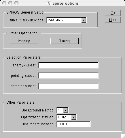
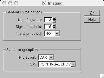
   5. Click on ``Background options'' and un-select the flat-field option and select the ``Use tracers to model background'' option as shown in Fig. , and click "Ok" to close this window.

      Figure: Background GUI

      

   6. Back in the parent window click "spiros" to open the GUI window shown in Fig. .

      Figure: spiros GUI main window

      

   7. Make sure that the ``imaging'' mode is specified. Do not introduce any selection parameters, and specify the "Background method" and the "Optimization statistic". Background method "1" means that the background derived from the periods before and after the burst, and rescaled to the burst duration, will be subtracted from the burst data as a fixed background. With background method "3" the background will be scaled through the image deconvolution process, solving for a single background scaling coefficient. Do not use other options. For the "Optimization statistic", is recommended, while LIKEH can be tried in a second run. Click on "imaging" to check that the default parameters shown in Fig.  are correctly entered (and update them if necessary).

      Figure: spiros GUI imaging window

      

   8. Close all sub-windows by clicking twice "Ok", then using the "Save As" button, you can save the parameters you have just entered into a file. Enter the name ``grb_analysis.par'' and store it in the current directory. Please, make sure no spelling mistake is introduced. The GRB scripts read the file ``grb_analysis.par'' located in the current directory to load the analysis paameters.

   9. Once the parameters are ``saved'', click on ``Quit'' to quite the process. We do not want to run the analysis yet. This procedure is just a convenient way to enter parameters for the later analyses.

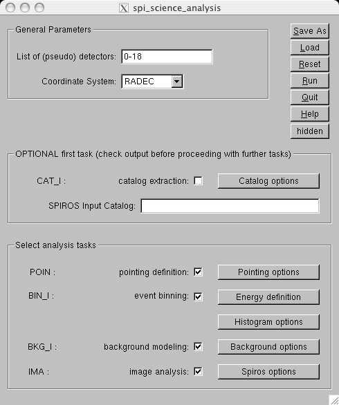
   If you do not want to use the GUI, you can also specify the above parameters by editing the spi_science_analysis.par file located in your $PFILES directory.

6. The ``grb_analysis.par'' file located in the current directory contains now the main parameters you want to use in your burst analysis. This file will be used by the script.

7. Run ``spi_grb_analysis''. Without any command line argument you get the following help text.

   Figure: Outputs of spi_grb_analysis when invoked without any input parameters

   

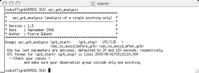
   You know the input parameters from the first point above, so you can then launch the spi_grb_analysis script. Make sure the "grb_start" - "sec_to_avoid_before_grb" is not before the pointing start, and that "grb_stop" + "sec_to_avoid_after_grb" is not after the pointing end, as there is no corresponding checks in the spi_grb_analysis script.

   In our example:

   spi_grb_analysis 2003-05-01T03:10:10.000 2003-05-01T03:10:30.000 UTC 10 10.

   You can re-run spi_grb_analysis in the same directory as many times as you wish, changing the parameters as explained above. However, when making a new run, the output of the previous run will be deleted. If you want to keep your output before making a new run, save them by copying the entire directory (e.g., cd ..; cp -r grb030501 grb030501_imaging; cd grb030501) before continuing.

8. "spi_grb_analysis" is calling a number of executables and "spi_science_analysis" several times. Since "spi_science_analysis" produces its own log file, the log file situation after running "spi_grb_analysis" is somewhat complicated. The resulting "spi_grb_analysis.log" is the high level log file, containing logs from the executables called directly by "spi_grb_analysis". In addition, you can find three log files ``spi_pointing.log'', ``spi_binning.log'', and ``spi_spiros.log''. The first contains the outputs of spi_obs_point, the second includes the logs from the binning to background steps, and the third contains the results from spiros.

9. After a successful execution of ``spi_grb_analysis'', it is also possible to run spiros again with the ``spi_science_analysis'' script. Launch ``spi_science_analysis'', make sure you select only the spiros step (if you select any other step, the burst background produced by ``spi_grb_analysis'' will be deleted and you will have to start it all again), change the required spiros parameters (making a LIKEH analysis rather than a one for example), and run the show again.