Starting with OSA 6.0, the spi_science_analysis script offers
phased-resolved analysis capabilities. The main switch is in the
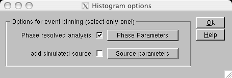
``Histogram options'' of the top-level GUI. Clicking on this button
opens a window shown in Fig. ![[*]](crossref.png) . This feature is not implemented in
spimodfit_analysis.
. This feature is not implemented in
spimodfit_analysis.
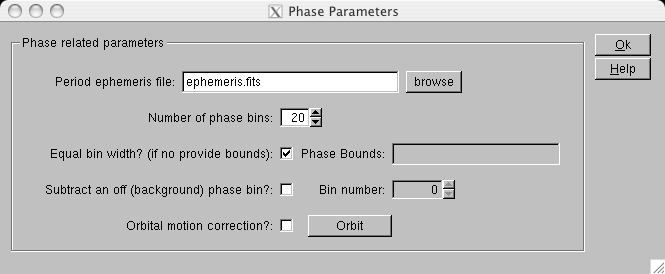
Open the ``Phase Parameters'' window (Fig. ) by
selecting ``Phase resolved analysis'' and clicking on ``Phase
Parameters''. The source ephemeris has to be provided through a FITS
file, the format of which is described in the next sub-section
(Sect. ). You can then specify the number of phase
bins. Equally spaced bins will be used by default, but if you
un-select ``Equal bin width'' you can provide specific phase bounds.
Be careful when entering this parameter as it may seem confusing. Here
is an example for the Crab of a phase bound vector with ``Number of
phase bins = 7'':
Phase Bounds = 0.00 0.03 0.20 0.38 0.50 0.80 0.98 1.00
``Phase Bounds'' must include values between 0 and 1, and it must start with 0 and end with 1. However, the first bin (0 to 0.03) and the last bin (0.98 to 1.00) will be merged in the program, resulting in a phase bin -0.02 to 0.03, or equivalently 0.98 to 1.03 one period later. Therefore, the above example is a 6 phase bin analysis despite the ``Number of phase bins = 7''. The number and boundaries of the phase bins are clearly written in the logfile, that you should consult in case of any doubt (see below).
The following parameter ``Subtract an off phase bin'' allows to specify an off-pulse phase bin number. The counts from the off-pulse phase bin will be subtracted to the counts of all other bins, after being properly scaled to their actual phase bin sizes. The phase bin are numbered starting with 0. This option can be used with regularly or irregularly spaced bins, although in general an off-pulse phase bin will have to be defined using specific bounds. Do not forget that in the case that the first and last bins are merged (see above).
Below is the log file output for the above case. Again the parameter ``Number of phase bins'' is 7 in this example, 8 ``boundaries'' are provided, but it is a 6 phase bin case in reality (numbered from 0 to 5). In this case, ``Subtract an off phase bin'' was also selected with a ``Bin number'' equal to 4.
Number of phase bin ..............: 6
Phase bin No  0 : from 0.000000 to 0.030000 and from 0.980000 to 1.000000
Phase bin No 1 : from 0.030000 to 0.200000
Phase bin No 2 : from 0.200000 to 0.380000
Phase bin No 3 : from 0.380000 to 0.500000
Phase bin No 4 : from 0.500000 to 0.800000
Phase bin No 5 : from 0.800000 to 0.980000
Counts from phase bin 4 will be subtracted from all spectra
If you select ``Equal bin width'', the parameters are less confusing, and with a ``Number of phase bin = 5'' the log file contains the following outputs.
Number of phase bin ..............: 5
Phase bin No 0 : from 0.000000 to 0.200000
Phase bin No 1 : from 0.200000 to 0.400000
Phase bin No 2 : from 0.400000 to 0.600000
Phase bin No 3 : from 0.600000 to 0.800000
Phase bin No 4 : from 0.800000 to 1.000000
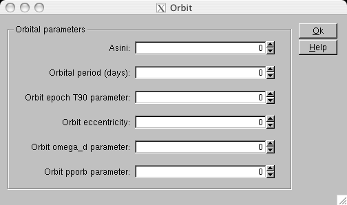
Finally, an orbit can be specified in the case of a source with a
companion in a binary system by entering the orbit parameters in the
``orbit'' window (Fig. ). Use zero values if there is no
orbital constrains in your analysis.
The phase-resolved analysis is then executed after you have clicked three times on ``Ok'' buttons. The binning step produces one set of detector spectra for each phase bin, called ``evts_det_spec_phase_i.fits'' where i is the phase bin number. Note that these files named ``spec'' or ``spectra'' are our particular format to store binned events but that these ``count spectra'' may comprise only one energy bin in case of imaging analysis.
The next background step is phase bin independent (since the background is eventually scaled to the data in the image reconstruction), and consequently it is executed only once. spiros is run independently for each phase bin in turn and one set of results is produced for each bin. Again spectra and their index are numbered by introducing a ``phase_i'' to the file names used for phase independent analyses, where again i is the phase bin number. The same RMF response file (spectral_response.rmf.fits) is valid for all phased-resolved spectra (and automatically attached to them), and therefore the XSPEC spectral fitting of these spectra is straightforward.