Spectral Extraction using spimodfit

First, set-up the environment and create the observation group as detailed in the sections for spi_science_analysis. Then select a suitable catalogue for the observation you are analyzing. Using the cook book example, the name is source_cat.fits, and you may leave this name. In our example we set the column FLAG to the value 1 only for the Crab. Launch spimodfit_analysis and select the steps. You can skip the background step, since spimodfit handles it internally.

Figure: GUI of spimodfit_analysis with the default setting.

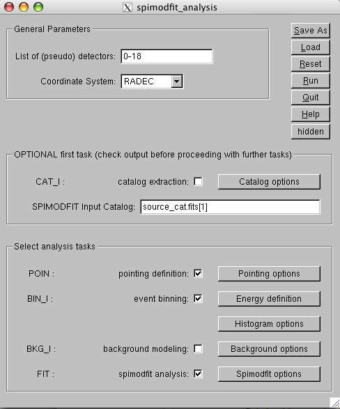
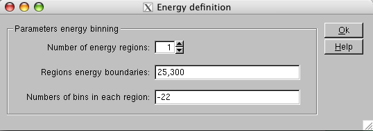
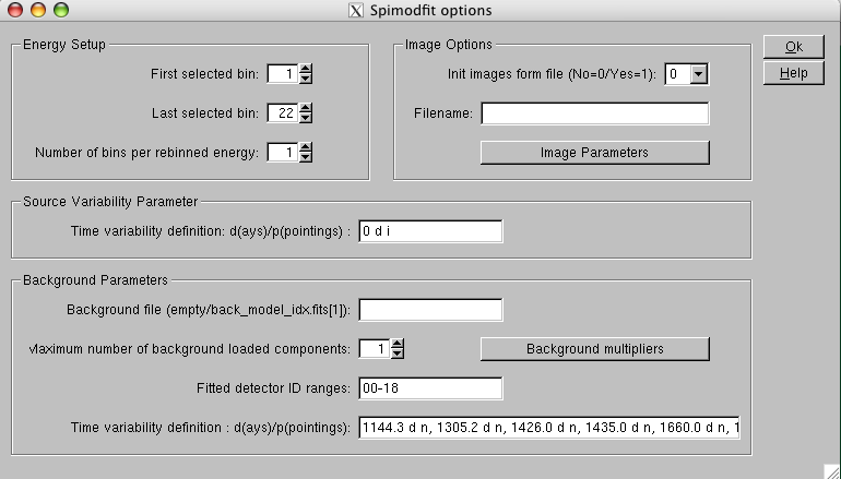
Now click on the energy definition options and select the number of channels you want in the final spectrum. We chose 22 logarithmic bins from 25 and 300kev (Fig.) in our example. Close this window, open the window on ``spimodfit options'' (Fig. ) and choose correctly in the upper left frame the selected bins according to your binning choice. You can rebin at this stage with an integer number of bins. All the other parameters can be left to the default values.

Figure: GUI of spimodfit_analysis energy definition.

Figure: GUI of spimodfit_analysis regarding spimodfit .

Several files are produced as output. One should check the fit quality through, e.g., the log file spi_sa_DATE.log, where DATE is the start time of the analysis. For each energy range, there is the value of the and of the statistics at optimum. These should be around one. If a is obtained, a warning is issued and the user should consider to vary the input catalog and/or the variability time scales.

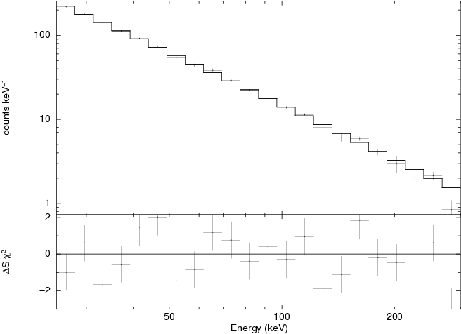
For the user interested in spectral analysis of point sources the relevant output are the spectra named spectrum_SRC.fits and the response matrix spectral_response.rmf.fits. No ancillary effective area is necessary. In our case the Crab spectrum is (spectrum_Crab.fits) whose fit with a power law yields a spectral index and normalization at 1keV (Fig. ). The response matrix is computed by the script spimodfit_rmfgen.csh, which should be run manually in case the file spectral_response.rmf.fits is not present.

Figure: Count rate spectrum of the Crab from the cookbook example and the residuals from the best fit model.

To run the fitting step another time the script automaticcaly deletes the previous output files with the command

rm -f spimodfit\_*

therefore if the user wants to compare the results of subsequent runs, he/she should copy the relevant files elsewhere. At odds with the spi_science_analysis pipeline, the results of spimodfit are not attached to the og_group, therefore the deletion of these files does not produce any harm to the og_tree.