When og_create has finished without any errors, move from the top-level directory ($REP_BASE_PROD) into the analysis directory (``./obs/spi_analysis/'') and launch the spi_science_analysis script
cd obs/spi_analysis
spi_science_analysis
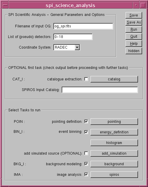
After a few seconds the GUI will appear, provided that the DISPLAY environment variable is set properly, otherwise you will be prompted for the individual parameters on the command-line. In general, but especially for learning SPI data analysis, we strongly recommend using the GUI.
The top section holds the most basic parameters of the pipeline, the list of detectors which are to be used in the analysis and the coordinate system. Do not change the default values for the current example analysis.
The middle section concerns
the catalogue extraction/specification part. For most of the bright
sources, the available catalogue source positions![[*]](footnote.png) are more accurate than
the positions which can be derived from the SPI data (due to the
limited spatial resolution). The best results are therefore obtained
by fixing the known source positions in the image reconstruction
process. However, as some sources are highly variable and the
catalogue fluxes not always reliable, it is sometimes difficult to
predict which sources will be detected in a given observation. In
order to avoid specifying wrong positions (where no significant
sources can be detected), it is a good idea to first explore your data
set and see which sources can be detected without using any prior
information. Un-select the ``catalogue extraction'' and leave the
``spiros input catalogue'' entry empty (we explain how to use the
catalogue in next Sect.
are more accurate than
the positions which can be derived from the SPI data (due to the
limited spatial resolution). The best results are therefore obtained
by fixing the known source positions in the image reconstruction
process. However, as some sources are highly variable and the
catalogue fluxes not always reliable, it is sometimes difficult to
predict which sources will be detected in a given observation. In
order to avoid specifying wrong positions (where no significant
sources can be detected), it is a good idea to first explore your data
set and see which sources can be detected without using any prior
information. Un-select the ``catalogue extraction'' and leave the
``spiros input catalogue'' entry empty (we explain how to use the
catalogue in next Sect. ![[*]](crossref.png) ).
).
Select the pointing definition, event binning, background modeling, and image analysis tasks, and click on the corresponding buttons to specify task specific parameters.
), you have
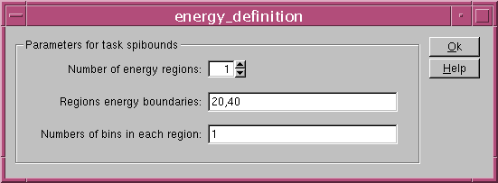
three parameters. In the first field, you can define a number of
energy regions. In the second one, you specify the actual limits in
keV of these regions, e.g., 20,40,60 is for two regions: 20-40keV
and 40-60keV. In the third field, you provide the number of bins
for each energy region (positive numbers provide linear scaling,
negative numbers logarithmic scaling). This allows for a more
elaborate definition of the binning than a simple logarithmic or
linear binning over the whole range. If you want gaps (e.g.,
20-40keV and 80-100keV) in your binning, you can simply set the number
of bins in the region in-between to 0.
For our example, we use a 20-40keV energy region, with one bin.
.
In this example, we use the default flat field option, which is recommended by the SPI team. Pre-defined flat-field spectra are available in the ic/spi/cal/ directory of the REP_BASE_PROD. They were derived by binning in 0.5 keV bins all events from empty-field observation revolutions:
The files above have been created recently (March 2018), hence they might not be available in your ic/spi/cal/ directory of the REP_BASE_PROD. To download or update the IC files see http://isdc.unige.ch/integral/analysis#Software
These spectra are rebinned in this step to match the bin size of your
analysis, and the program will select and use the appropriate
flat-field spectrum automatically. However, the temporal proximity criterion used in the pipeline
might not be the optimal one.
In case of bad fitting results, the user is encouraged to choose another flat-field
for the ``flatfield DOL'' in the panel of Fig. (an appropriate path is required).
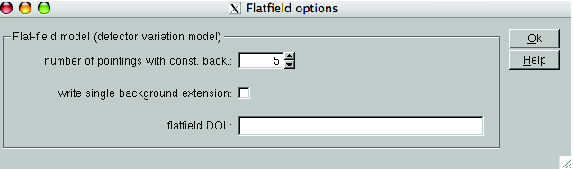
Within the flat field option, the detector to detector ratios are kept fixed (from that of the empty field), but one background coefficient is derived through the imaging reconstruction process. In fact, one coefficient is derived for each time interval, and the length of the intervals is provided as a number of consecutive pointings by the user.
To use the flat field model, select the flat
field in the main background GUI and press the button for the flat
fields options. Provide the number of pointings for which you assume
the background to be constant. Use a value of 5 in this example and
leave the ``write single background extension'' unselected. Note
that in general, much longer time interval can be used in the range 20
to 100 pointings. The ``write single background extension'' must only
be selected when using spimodfit instead of spiros
(see the section on spimodfit, Sect. ).
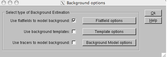
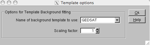
Another possibility to model the background accurately is to use background templates (the second option in the main background GUI). The background templates are provided by the SPI instrument team in Toulouse. These templates are derived from background tracers, but are fine tuned by the instrument specialists. Several templates exist based on various background tracers. A typical template is the GEDSAT which is based on the count rate of the events saturating the Germanium detector electronic (hence the name of the template). Other templates are based on the detector count rate, the non saturated events, and many more. The user is encouraged to try the various models to see which work best for his specific analysis and/or dataset. For typical point source analysis, a good starting point is the GEDSAT template. To use this model, un-select in the main background GUI the flat field option and select the background templates. Press the button for the template options and select the template to use.
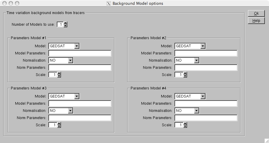
The background can be modeled through the direct use of background
tracers (the third option in the main background GUI). The GEDSAT
model, which is also based on the count-rate of the events saturating
the Germanium detector electronic is a good alternative to model the
background. In this case, un-select the flat-field option and select
the tracers option in the main background GUI. Press the Background
model options button to set the options. Set the ``Number of Models to
use'' to 1, and select the GEDSAT model. For more complicated setups
you can use more components. The GUI offers the possibility to use up
to four different model components simultaneously. In the image
reconstruction process, we will assume that the real detector
background varies in the same way as this model, which will be scaled
to the actual data to determine the real background. GEDSAT is a good
model for most point-source analyses (see Sect. for
more information about background modeling).
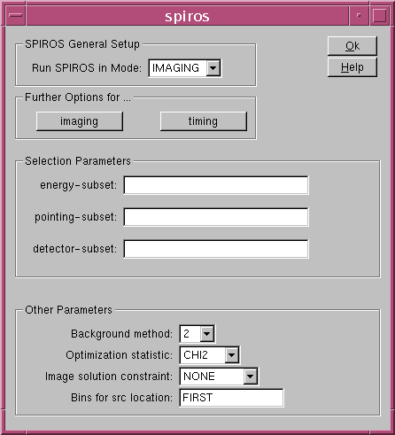
In the ``Selection Parameters'' field of the spiros GUI, you can specify three subsets of energy bins, pointings and detectors. If you leave the fields empty, spiros will use all data, otherwise only the specified energy bins, pointings, and detectors will be taken into account in the analysis. You can automatically ignore obviously bad data points by entering ``AUTO'' in the pointing subset. You can also use the AUTO filter in addition to specifying the pointings to use. For example, ``AUTO,5-25,30-50'' will use pointings 5-25 and 30-50 and apply the AUTO filter to these pointings. All other pointings will not be used.
The bottom section allows you to choose the ``Background method'', the ``Optimization statistic'', and the ``Bins for src location''.
For the background method, you must use method 3 if you selected the ``flat-field'' model. If you are using the GEDSAT model use method 2 (you can also use background method 5, also known as ``mean count modulation model'' (MCM), but be aware that this method may produce wrong results if you have bright variable sources in the FoV).
With spiros background method 3, one background scaling coefficient is derived for each time interval (specified as a number of pointings in the background model step) assuming that detector to detector background variations follow those from the flat-field model.
With spiros background method 2, one background scaling coefficient
is derived for each detector in the image reconstruction process. In
this way, we assume that the background variations in all detectors
follow that of the background model (see Sect. or the
spiros User Manual for more explanations).
For the optimization statistic, you can choose between maximum likelihood or . The latter is faster and more robust but can be problematic if you have lots of energy bins with zero counts. For imaging in broad energy bands, is definitely better, while you might want to compare results obtained with and likelihood options when extracting spectra.
The bins for source location determines in which energy bins spiros locates the sources. The typical setting will be ``FIRST'' where spiros uses just the first energy bin. But you may also use ``ALL'', where spiros will search for sources in each bin independently, or you may give a range of bins to be used.
For our example, we use background method 3, as optimization statistic, and ``FIRST'' for the source location bins.
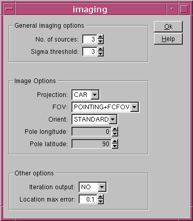
The options specific for imaging are available by clicking on the button ``imaging'' in the spiros GUI.
The top section allows you to select the maximum number of sources
you want spiros to look for (in addition to those that might be
provided through a catalogue, see Sect. ) and a lower
sigma threshold. spiros stops its iterative source search process
either when it has found the maximum number of sources or when the
sigma threshold has been reached. In our case, we ask spiros to
search for up to 3 sources with a detection significance larger than
3 sigma (enter 3 instead of the default 6).
We use the CAR (Cartesian) projection type for (almost) all cases. With the CAR projection the derived images have angular coordinates, with pixels regularly spaced by a constant angular step.
Since SPI is a coded mask instrument, you have to define the image
FoV, i.e., the sky region that spiros should
``reconstruct''. An easy way to specify the image FoV is to use the
POINTING option. The output image will then range from the minimum
to the maximum of the central latitude/longitude values of all
pointings included in your observation. Using ``POINTING+FCFOV'' or
``POINTING+ZCFOV'' will add half of the SPI fully-coded or
zero-coded FoV, respectively, on each side of the image defined by the pointing
centers. ``POINTING'' or ``POINTING+FCFOV'' produces the nicest
intensity images, but be aware that strong sources just outside your
image FoV can completely bias your analysis (see
Sect. ) and is therefore only recommended when no further
sources are close to the current FoV. Otherwise, if you suspect there exist
sources close to the FoV which may affect the reconstruction process, the
``POINTING+ZCFOV'' is a good choice for most observations. However, in this case
the resulting intensity images need careful tuning in ds9.
When the setup is done, click twice ``Ok'' (once on ``imaging'' and once on ``spiros''), then ``Run'' the pipeline. Depending on the number of science windows, the histogram building and image deconvolution can take quite some time.
Once the pipeline is finished (no errors should be apparent), you will find in your directory, among other output files, the intensity, significance, and error image files in FITS format:
spiros_image_intensity_result.fits
spiros_image_sigma_result.fits
spiros_image_error_result.fits
Before examining these images, convert the output catalogue produced by spiros into a format usable by ds9:
cat2ds9 "source_res.fits" source_res.reg

ds9 spiros_image_intensity_result.fits -region source_res.reg

ds9 spiros_image_sigma_result.fits -region source_res.reg
In our analysis example, and after adjusting appropriately the images with ds9, the resulting intensity and significance images should look like this:
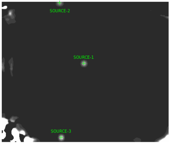
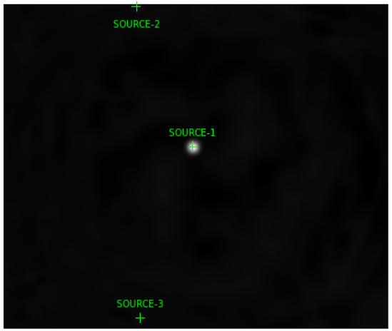
There are three sources in these images. In addition to the obvious, strong Crab detection, spiros has found two spurious sources with very low significance. In most cases, spiros does find spurious sources with detection significance in the range 3 to 5 sigma. Great care should be taken to make sure that sources with such detection significance are indeed real, and if you only want to see sources detected ``beyond any doubt'' raise the spiros lower sigma threshold to higher values (6 or 7 is usually a good choice).
The output file
source_res.fits
provides quantitative results formatted as a FITS table. You can open this file with, e.g., the ftool ``fv'':
fv source_res.fits
The resulting spiros Crab position is RA=83.617 DEC=22.019, while the catalogue position is RA=83.612 DEC=21.994. The difference is of the order of 1.7arcmin. As expected for very high S/N sources, this value is much smaller than the SPI spatial resolution. The Crab flux in this 20-40 keV energy band is ph/sec/cm , corresponding to a detection significance of 154. You can also see that the detection significance of the spurious sources is 6.4 and 5.8.
All these results can also be viewed, perhaps more conveniently, at the end of the log file (called spi_sa_``UT date''.log), below the following title
================================================================================
=                                                                              =
=        Summary of results from SPIROS-9.3.6 in IROS analysis mode            =
=                                                                              =
================================================================================
where you find the most important information about the analysis, such as the sources found at each iteration and information about the resulting images.