Before starting, you may want to save your imaging analysis again, by copying the current directory
cd ..
cp -r spi_analysis  spi_imaging_with_catalogue
cd  spi_analysis
Spiros program can only extract spectra at fixed, known positions. Therefore, a source_cat.fits file must be provided in any case. We assume that you have created/checked a source_cat.fits as explained in last section. Launch ``spi_science_analysis'', un-select the catalogue extraction step, and provide the input catalogue name source_cat.fits in the ``spiros input catalogue'' field.
It is not necessary to run the pointing step again. However, the number of considered energy bins is typically much larger in spectral extractions than in imaging reconstructions. Select the binning, background, and spiros steps. In the energy binning step, you can now select a binning suitable for a spectrum of a bright source with a broader energy range and a relatively high number of bins. For our example, set the number of regions to "1", a "20,1000" keV boundary, and " " as the number of bins. As stated before, using a negative bin number implies a logarithmic binning, with 100 bins from 20keV up to 1MeV in our case.
Open the spiros GUI and set spiros mode to spectra instead of imaging. Click ``Ok'' and ``Run'' the pipeline. After spiros has finished successfully, the pipeline will automatically generate the appropriate response matrix and attach it to your spectra.
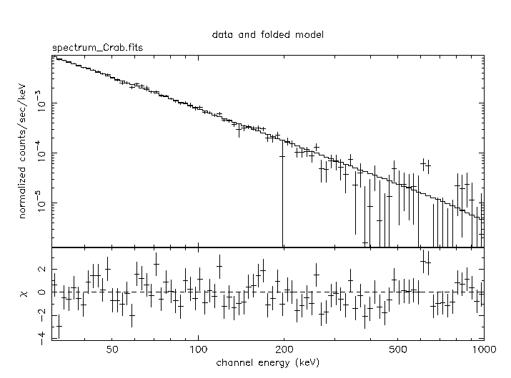
To evaluate the obtained results, you can use XSPEC to analyze your spectra. In the following example we fit a single power law from 30 to 1000keV. Here is a verbatim of the XSPEC session.
================================================================================

              Xspec 11.3.1    17:41:21 26-May-2005

For documentation, notes, and fixes see  http://xspec.gsfc.nasa.gov/

Plot device not set, use "cpd" to set it

Type "help" or "?" for further information
XSPEC>data spectrum_Crab.fits
POISSERR keyword not found, assuming FALSE
Net count rate (cts/s) for file   1  0.3903    +/-  3.3501E-03
  using response (RMF) file...       spectral_response.rmf.fits
  1 data set is in use
XSPEC>cpd /xs
XSPEC>setp en
XSPEC>plot ld
XSPEC>ign **-30.
ignoring channels     1 -    11 in dataset     1
XSPEC>model power
 Model:  powerlaw<1>
Input parameter value, delta, min, bot, top, and max values for ...
                  1      0.01        -3        -2         9        10
1:powerlaw:PhoIndex>
                  1      0.01         0         0     1E+24     1E+24
2:powerlaw:norm>
 ---------------------------------------------------------------------------
 ---------------------------------------------------------------------------
 Model:  powerlaw<1>
 Model Fit Model Component  Parameter  Unit     Value
 par   par comp
   1    1    1   powerlaw   PhoIndex            1.00000     +/-   0.00000
   2    2    1   powerlaw   norm                1.00000     +/-   0.00000
 ---------------------------------------------------------------------------
 ---------------------------------------------------------------------------
Chi-Squared =      4010090.     using    89 PHA bins.
Reduced chi-squared =      46092.99     for     87 degrees of freedom
Null hypothesis probability =  0.00
XSPEC>fit 50

<---snip--->

 ---------------------------------------------------------------------------
 Model:  powerlaw<1>
 Model Fit Model Component  Parameter  Unit     Value
 par   par comp
   1    1    1   powerlaw   PhoIndex            2.16210     +/-  0.123967E-01
   2    2    1   powerlaw   norm                13.3916     +/-  0.626640
 ---------------------------------------------------------------------------
 ---------------------------------------------------------------------------
Chi-Squared =      115.7470     using    89 PHA bins.
Reduced chi-squared =      1.330425     for     87 degrees of freedom
Null hypothesis probability = 2.137E-02
XSPEC>plot ld de

================================================================================
The final ``plot ld de'' produces the following spectral display.
Note that the remaining deviations are indeed really small, especially considering that we are using only 10 science windows in this example which is a very small number for SPI.