The numerical code used in this tool reproduces both synchrotron and Inverse Compton processes. Both the web interface and the numerical code have been developed by Andrea Tramacere. The numerical code has been used in several refereed publications, If you use this code in any kind of scientific publication you shall cite the following papers:
In the following is given a brief description of what blazars are, of the physical processes reproduced by the SED tool, and a user guide to the use of the web interface. To have a deeper understanding of the numerical code and of its physical implications we remand the reader to the references listed above.
Content:
A schematic view of
Blazars
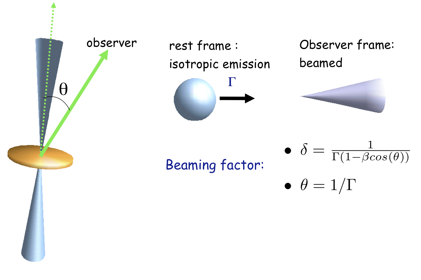
Blazars objects are Active Galactic Nuclei (AGNs) characterized by a polarised and highly variable non-thermal continuum emission extending from radio to γ-rays. In the most accepted scenario, this radiation i s produced within a relativistic jet that originates in the central engine and points close to our line of sight. Since the relativisti c outflow moves with a bulk Lorentz factor (Γ) and is observed at small angles (θ ≃ 1/Γ ), the emitted fluxes are affected by a beaming factor δ = 1/(Γ(1 − βcos θ )) . To model the emission processes we assume to have a plasma of leptons (e+/-) distributed in a one-zone homogeneous emitting region. This emitting is assumed to have a spherical geometry, and an entangled magnetic fie lds. The electron are accelerated to relativistic energies (through shock firs order, or stochastic second order acceleration), and their energy distribution is described by an analytical law. These accelerated electrons interact with the entangled magnetic field, and emit synchrotron radiation.
 In the case of synchrotron self Compton model (SSC)(Jones et al. 1974) the
seed photons for the Inverse Compton (IC) process are the synchrotron photons
produced by the same population of relativistic electrons. In the case of
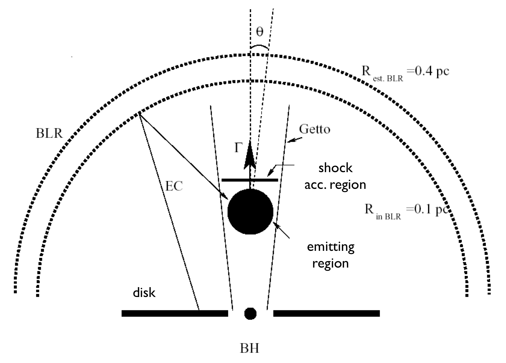
external radiation Compton (ERC) scenario (Sikora et al. 1994),
the seed photons for the IC process are typically UV photons generated by the
accretion disk surrounding the black hole, and reflected toward the jet by the
Broad Line Region (BLR) within a typical distance from the accretion disk of
the order of one pc. If the emission occurs at larger distances, the external
radiation is likely to be provided by a dusty torus (DT) (Sikora et al. 2002).
In this case the photon field is typically peaked at IR frequencies.
In the case of synchrotron self Compton model (SSC)(Jones et al. 1974) the
seed photons for the Inverse Compton (IC) process are the synchrotron photons
produced by the same population of relativistic electrons. In the case of
external radiation Compton (ERC) scenario (Sikora et al. 1994),
the seed photons for the IC process are typically UV photons generated by the
accretion disk surrounding the black hole, and reflected toward the jet by the
Broad Line Region (BLR) within a typical distance from the accretion disk of
the order of one pc. If the emission occurs at larger distances, the external
radiation is likely to be provided by a dusty torus (DT) (Sikora et al. 2002).
In this case the photon field is typically peaked at IR frequencies.back to content
The Parameters Menu
This menu is used to provide the SSC/EC model parameters. It's organized in the following sections, each correspondingo to a form:
- The Jet form description
- The n(γ)
form description
- The Emission scenario form description
- Caveat on accretion diks parameters
- The Run Model buttom
To run the model the user has to click on the "Run Model" button.
The Jet form description
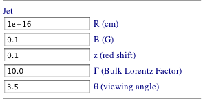
- R: the size of the spherical emitting region in cm
- B: the intensity of the entangled magnetic field (expressed in Gauss) within the emitting region with size R
- z: the redshift of the host galaxy
- Γ: the Bulk Lorentz factor of the emitting region
- θ: the Jet viewing angle
the corresponding beaming factor of the jet will be :δ = 1/(Γ(1 − βcos θ
)).
The n(γ) form description
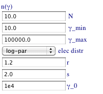
1=\int_{\gamma_{min}}^{\gamma_{max}}Kf(\gamma)d\gamma
in this way, by defining the differential electron distribution function n(γ) as:
n(\gamma)= N K f(\gamma)
the numerical value N will provide, by definition, the number of emitting particles per unit volume expressed in #/cm3:
- power-law:
a power law function, defin as:
f(\gamma)=\gamma^{-p}- p = spectral index
- pl+exp cutoff:
power law function plus an exponential cutoff, definided as :
f(\gamma)=\gamma^{-p} exp(-\gamma/\gamma_{cut})- p = spectral index
- γcut = cut off energy
- log-par:
a log-parabolic funtion defined as :
f(\gamma)=(\gamma/\gamma_0)^{-(s+r\log(\gamma/\gamma_0))}- γ0 = reference energy
- s = spectral index at the reference energy γ0
- r = spectral curvature
- log-par+pl:
a log-parabolic funtion plus a power-law low energy branch, defined as:
f(\gamma)=(\gamma/\gamma_0)^{-s}, \gamma \leq\gamma_0f(\gamma)=(\gamma/\gamma_0)^{-(s+r\log(\gamma/\gamma_0))}, \gamma >\gamma_0
- γ0 = energy at which pl turns int log-par
- s = spectral index at the reference energy γ0
- r = spectral curvature
- log-par Ep:
a log-parabolic function, described in terms of peak energy and peak curvature, defined as :
f(\gamma)=10^{-(r\log(\gamma/\gamma_p)^2)}- γp = energy at which pl turns int log-par
- r = spectral curvature
-
broken pl:
a broken power law function, defined as:
f(\gamma)=(\gamma)^{-p}, \gamma\leq \gamma_{break} \\f(\gamma)=(\gamma)^{-p1}, \gamma> \gamma_{break} \\- p = low energy spectral
index
- γbreak =
break energy
- p1 = high
energy spectral index
- p = low energy spectral
index
The Emission scenario form description
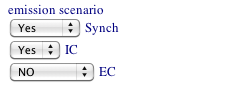
- Synch drop-down:sets the synchrotron
emission
- yes = synchrotron emission is computed
- Self-ab= synchrotron self absorption is computed
- no = synchrotron emission is not computed
- IC drop-down: sets the inverse
Compton (SSC) emission
- yes = IC emission of synchrotron photons (SSC) is computed
- no = IC emission of synchrotron photons (SSC) is not computed
- EC drop-down: sets the External emission
- BLR = computation of EC emission disk
seed photons reprocessed by the Broad Line Region (BLR)(read the caveat ont
accretion disk paramters)
- L_disk = disk luminosity in erg/s
- dist BLR disk = Radius of the BLR in cm
- τ_BLR = fraction of diks luminosity reflected by the BLR
- T_disk= peak disk temperature in Kelvin
- Dust = computation of IC emission of seed disk
seed photon originating in the dusty torus
- L_disk = disk luminosity in erg/s
- dist TORUS disk = radius of the dusty torus
- τ_DT= fraction of diks luminosity
re-emitted by the torus in the infrared
- T dust= dust temperature in
Kelvin
- Dust+BLR =
computation of EC emission both
for BLR and Dust
- BLR = computation of EC emission disk
seed photons reprocessed by the Broad Line Region (BLR)(read the caveat ont
accretion disk paramters)
Caveat on accretion diks parameters
To model the accretion disk we follow the approach of Ghisellini et al.
2009. In the following we explain how to link the input parameters (L_disk,T_disk), to the Black Hole (BH) mass,
to the accretion efficiency, and to the accretion rate. We start from the
relation expressing the accretion disk temperature as a funciont of the
distance (R) from the BH, as function of the accretion efficiency ε,
of the Schwarzschild radius (RS), and of the disk luminosity
(Ldisk):
this function peaks at R4RS, with a temperature Tdisk, hence we can derive RS as :
where we use a reference value of ε=0.1. From RS it is straightforward to derive the BH mass (RS = 2 GMBH/c2), and from the relation:
we can derive the accretion rate.
back to content
The Run Model buttom

By clicking on this buttuon the SSC/EC model is computed, according to the paremters inserted in the forms above. The output will be shown in the right frame.
If the "save model" radio button is
cheked, after the model computation, at the side of the SED plot will appear a
link to save the model file, corresponding to the computation. This file can be
uploaded later, using the Upload Menu
The working area menu description

The user can decide to set a working directory on the remote machine, and a flag, in this way it's possible to store different results organized in directories (path), and in the same directory with different names (flag) :
- "path"
- the name
of the directory to create on the remote machine
- the name
of the directory to create on the remote machine
- "flag"
- the name for the output files of the current model
The Upload menu description

By using this meny, the user can upload a spectral energy distribution, or
a model file saved fro a previous computation. These two options can be chosen
by the following form:
- "Load Data File": The user can upload an SED using an ascii file, with the following format:
- if plot type = "observed"
- freq = νrest
- flux = νobsFobs
- if plot type = "rest frame"
- freq =νobs
- flux = νrestLν rest
- "Load Model File": The user can upload a model file where has saved the parameters of a previous computation. To save a Model file, check the "save model radio button" in the Submit menu, and download the corresponding model file using the link that appears close to the SED plot:
back to content
The Plot menu description
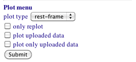
The plot menu is used to set plotting options. The output will be shown in the right frame. The "plot type" drop down menu allows to choose betwen :
- "observed"
- "rest-frame"
- frequencies are transformed according to: νrest = νobs /(1+z)
- fluxes are transformed to
luminosities according to:
νrestLν rest = 4πD2L νobsFobs
where DL is the luminosity distance
There radio buttons allows to select different plotting options:
- "only replot": in this case will
be only updated the plot, the SED model will be not updated. For example,
you may upload an SED file to plot on top of your model
- "plot uploaded data": in this
case the uploaded SED will be plotted
- "plot uploaded data": in this
case "only" the uploaded SED will
be plotted
References:
Jones et al. 1974Ghisellini et al. 2009
Massaro E. et al. 2004
Massaro E. et. al 2006
Sikora et al. 1994
Sikora et al. 2002
Tramacere A. et al. 2007
Tramacere A. et al. 2011
Tramacere A. et al 2009