Spectral Extraction

It is not possible to extract the spectrum of only the source you are interested in. All sources brighter or compatible with the one you are interested in should be taken into account too. Thus it is strongly recommended, when you deal for the first time with your data, to run the analysis until the IMA level, as described in Section , check the results, and call ibis_science_analysis once again to run the spectral extraction part. The description of the algorithm used for spectral extraction is given is Section .

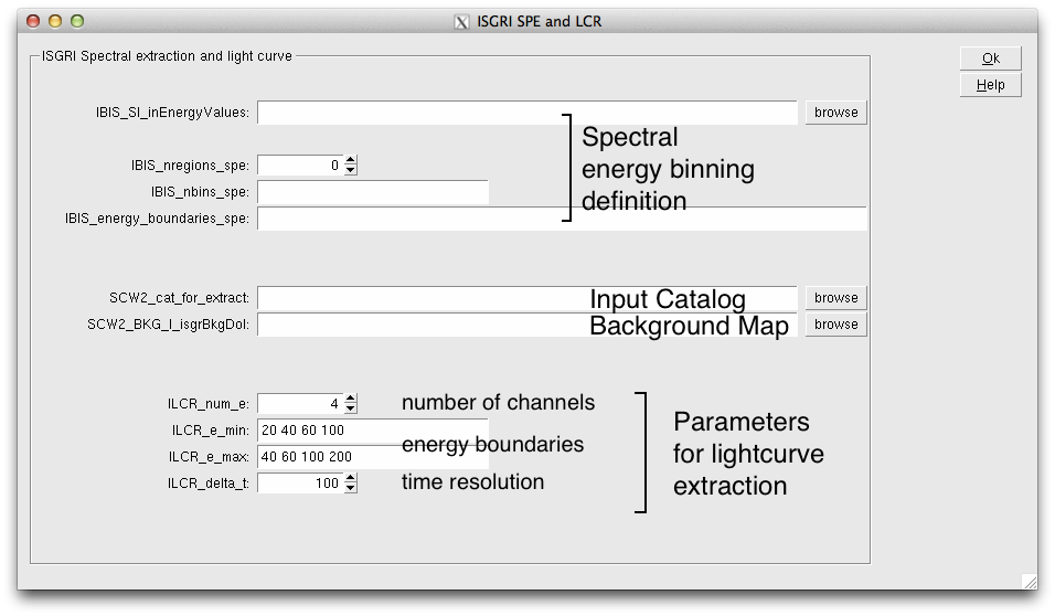
Launch ibis_science_analysis, and on the main GUI page change Start Level to BIN_S, and End Level to SPE. After that press the ISGRI SPE and LCR button.

Figure: Page of IBIS GUI for Spectral and Ligtcurve extraction

On the screen that appears (see Figure ), you can specify:

Spectral energy binning:
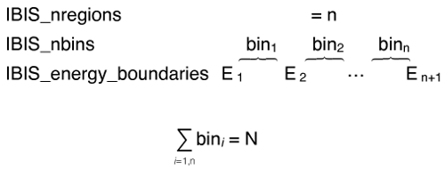
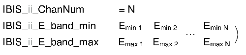
With OSA11.0 we introduced a new way to define the energy bins: this can now be achieved more conveniently through the new parameters: IBIS_nregions_spe, IBIS_nbins_spe, and
IBIS_energy_boundaries_spe, as explained in the sketch of Fig. , and detailed in Sect. .

Alternatively, with the help of the parameter IBIS_SI_inEnergyValues you can specify the file (and its extension) describing the desired binning of the response matrix.

Starting from OSA11.0 we are also introducing multpile Response Matrix Files. Each of these files is valid only for a set of contiguous revolutions, with time granularity depending on the response evolution, whereas previously we were using a single RMF covering the entire mission. Our software automatically selects the RMF files corresponding to your observation and rebins it according to the energy binning that you defined.

Figure: Energy binnings can be defined through either one of the above parameter sets, for spectra as well as for imaging (here we put only the common part of the parameter name. For example you should use IBIS_II_ChanNum or IBIS_nregions_ima for imaging; and IBIS_SI_ChanNum or IBIS_nregions_spe for spectral analysis).

Background maps:
With the SCW2_BKG_I_isgrBkgDol parameter you can specify the background map to be used in the spectral and timing analysis. It is recommended to use the same background map as in the imaging case. Default empty value corresponds to the default map ($REP_BASE_PROD/ic/ibis/bkg/isgr_back_bkg_0011.fits).

Input catalog for Spectral and Lightcurve extraction:
By default a spectrum will be created for all sources listed in the isgri_srcl_res.fits catalog created during the IMA step. The position of the source will be taken from RA_FIN, DEC_FIN columns. Note however that spectral extraction is time consuming, and it is not recommended to include sources that are faint in comparison with the source of interest.Copy isgri_srcl_res.fits to another file, say specat.fits as shown below, leaving only sources with significance higher than a threshold ( in the example below):

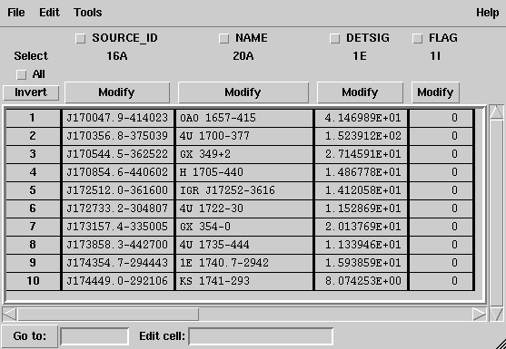
cd  $REP_BASE_PROD/obs/isgri_gc
fcopy "isgri_srcl_res.fits[ISGR-SRCL-RES][DETSIG >= 7.0]" specat.fits

(Note, that there should be spaces around " ").

Note that it is important to make the resulting catalog read only:

 chmod -w specat.fits

Part of the resulting specat.fits catalog is shown in Figure .

Figure: List of sources used for the spectral analysis

The same catalog will be used later for the lightcurve extraction.

In the GUI, set the SCW2_cat_for_extract parameter to point to specat.fits (use the browse button to get the full path) and press Ok, the window disappears and you are back to the main GUI page. There, press Run to launch the analysis.