Timing Analysis without the Deconvolution

Read this if you are interested in fast variability studies (up to milliseconds).

In this section we describe a way of doing timing analysis in a non binning way, i.e. starting from the single events. This way is suitable for very short time scales (up to milliseconds) and is less recommended for long time bins for which the binning tools ii_light and ii_lc_extract are suitable.

In the text we will use one of the Science Windows with Crab data you have downloaded to run the PICsIT analysis (e.g. 003900020020).

In general the table with the events is very big, so if you are interested in only part of the Science Window (e.g. in the case of a burst) it is better to define a user good time interval (see Section 9) and work within it.

To select the photons that come from a given source in the field of view, you need to have the corresponding PIF. PIF is automatically created during the SPE step, but can also be created with a standalone tool ii_pif.

Create with og_create observational group $REP_BASE_PROD/obs/crab/og_ibis.fits, and run analysis from COR to DEAD level, prepare the catalog, with Crab only and run ii_pif.

Figure 22: Crab power spectrum.

cd $REP_BASE_PROD/obs/crab
ibis_science_analysis ogDOL="./og_ibis.fits" startLevel=COR endLevel=DEAD 

fcopy infile="$ISDC_REF_CAT[NAME=='Crab']" outfile="crab_specat.fits"

ii_pif inOG="" outOG="og_ibis.fits" inCat="../../crab_specat.fits"\
        num_band=1 E_band_min="20" E_band_max="1000"\
        mask="$REP_BASE_PROD/ic/ibis/mod/isgr_mask_mod_0003.fits"\
	tungAtt="$REP_BASE_PROD/ic/ibis/mod/isgr_attn_mod_0010.fits"\
	aluAtt="$REP_BASE_PROD/ic/ibis/mod/isgr_attn_mod_0011.fits"\
	leadAtt="$REP_BASE_PROD/ic/ibis/mod/isgr_attn_mod_0012.fits"

Now you are ready to create the lists of photons

						
cd $REP_BASE_PROD/obs/crab
evts_extract group="og_ibis.fits" \
events="crabevts.fits" instrument=IBIS \
sources="crab_specat.fits" gtiname="MERGED_ISGRI" \
pif=yes deadc=yes attach=no barycenter=1 timeformat=0 instmod=""

To increase signal-to-noise ratio select only events with PIF=1:

fcopy "crabevts.fits[2][PIF_1==1]" crab_pif1.fits 
chmod -w crab_pif1.fits

Now you can produce the Crab power spectrum:

powspec
Ser. 1 filename +options (or @file of filenames +options)[] crab_pif1.fits
Name of the window file ('-' for default window)[] -
Newbin Time or negative rebinning[] 0.001
Number of Newbins/Interval[] INDEF
Number of Intervals/Frame[] INDEF
Rebin results? (>1 const rebin, <-1 geom. rebin, 0 none)[]  0
Name of output file[default]
Do you want to plot your results?[] yes
Enter PGPLOT device[] /XW
hardcopy crab_powerspec.ps/PS

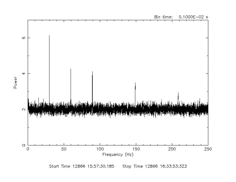
As a result, the crab_powerspec.ps plot, shown in Figure 22, was produced. The 33 millisecond pulsation of the Crab is visible. For the details on INTEGRAL absolute timing see Walter et al. 2003 [13].

If your data have many short GTIs (e.g. in the case of telemetry saturation due to a solar flare or when PICsIT is in non standard mode) you can obtain spurious results. A typical case is finding an 8sec period in your data due to the fact that the telemetry restart is synchronized with an 8sec frame! When possible, compare your results with ii_light that is immune to this problem and can reach about 0.1 sec binning.